
Average contig length times 1.6783469... is equal to N50
Probabilistic setup of sequence assembly outputs
When one analyzes sequence assemblies, a mysterious definition they inevitably encounter is the N50. N50 is commonly defined as the size \(L\) of the smallest contig such that summing all contigs of size \(\geq L\) gives at least half of the total sequence assembly length. The reason for using N50 intuitively is that we don’t want small contigs, of which there may be many, to skew the average contig length. See here or the Wikipedia article for more info.
Given a set of contigs coming from an assembly, how does the N50 relate to the average contig length? This may seem like a silly question because they aren’t related in general; you can easily come up with distributions of contig sizes with fixed average length and wildly varying N50s. However, I’ll show that under some (maybe not so mild) assumptions, the average contig length and N50 are related by a surprisingly simple formula.
Let’s make the following assumptions:
-
Assume that we have a fixed number of \(n\) contigs of size \(x_1,...,x_n\) and define \(\sum_{i=1}^n x_i = N\). Here \(x_1,..,x_n\) are the sizes of contigs output by an assembly, and \(N\) is our putative assembly length.
-
Assume that \(x_i\) are random, i.i.d, and exponentially distributed \(x_i \sim Exp(\frac{1}{\lambda})\) with mean length \(\lambda.\) Contigs have continuous, random size in our setup.
I chose an exponential distribution because contig lengths tend to have a heavy tail with a few large contigs and many small ones.
Under our probabilistic setup, the average length of the contigs is \(\mathbb{E}[x_i] = \lambda\), but can we calculate what the N50 is analytically?
Defining N50 probabilistically
First, let’s define the empirical N50 rigorously.
Definition: The empirical N50, \(\hat{N_{50}}\), is a random variable defined as the smallest \(x_j = \hat{N_{50}}\) where \(x_j \in \{x_1,...,x_n\}\) such that
\[\sum_{x_i \geq \hat{N_{50}}} x_i = \sum_{i=1}^n x_i \mathbb{1}_{x_i \geq \hat{N_{50}}} \geq \frac{N}{2}.\]This is just a mathematical generalization of the original definition of the N50 if you have a bunch of samples (i.e. contigs). Now I’ll introduce a probabilistic definition of the N50.
Definition: The N50 is a constant \(N_{50}\) satisfying
\[\mathbb{E}[\sum_{i=1}^n x_i \mathbb{1}_{x_i \geq N_{50}}] = \frac{\mathbb{E}[N]}{2} = \frac{n\lambda}{2}.\]The N50 is not a random variable, but a specific constant defined to satisfy an equation. Intuitively, the N50 is what we believe the value of empirical N50, \(\hat{N_{50}}\), should be when \(n\), the number of samples, gets really large. Notice that this is essentially a generalization of the probabilistic definition of the median and the empirical median. Here is a suggestive sketch of an argument that these two quantities are related.
Notice that
\[\frac{N}{2} + \max_{m=1,...,n} x_m \geq \sum_{x_i \geq \hat{N_{50}}} x_i = \sum_{i=1}^n x_i \mathbb{1}_{x_i \geq \hat{N_{50}}} \geq \frac{N}{2}\]follows after thinking about the definition of the empirical N50 for a bit. It turns that \(\mathbb{E}[\max_{m=1,...,n} x_m] = \sum_{i=1}^n \frac{1}{i} = O(\log n)\) is the nth harmonic number, see this explanation. Then taking expectations where \(\mathbb{E}[N] = n \lambda\) and dividing by \(n\), we get that
\[\frac{\lambda}{2} + o(1) > \frac{\mathbb{E}[\sum_{i=1}^n X_i \mathbb{1}_{x_i \geq N_{50}}]}{n} \geq \frac{\lambda}{2}.\]So \(\frac{\mathbb{E}[\sum_{x_i \geq \hat{N_{50}}} x_i]}{n} \rightarrow \lambda/2.\) Thus, from the definition of empirical N50,
\[\lim_{n \rightarrow \infty} \frac{\mathbb{E}[\sum_{i=1}^n x_i \mathbb{1}_{x_i \geq \hat{N_{50}}}]}{n} = \frac{\mathbb{E}[\sum_{i=1}^n x_i \mathbb{1}_{x_i \geq N_{50}}]}{n}.\]This is the reason behind the definition, and suggests that \(\hat{N_{50}} \rightarrow N_{50}\) is some sense, probably in probability.
I haven’t tried too hard to prove that \(\hat{N_{50}} \rightarrow N_{50}\) as n gets large. The proof should probably be similar to the proof that the empirical median converges to the true median. In my simulations, it seems to be the case that \(\mathbb{E}[\hat{N_{50}}] \rightarrow N_{50}\), so let’s just assume that these quantities are related for the rest of the post. Maybe someone else can take a stab at it; let me know how it goes!
Calculating the N50
Let’s define \(\sigma = N_{50}\) for the rest of the post, for ease of notation. We can actually calculate the N50 as follows. Because \(\sigma\) is a constant, \(x_i \mathbb{1}_{x_i \geq \sigma}\) are identically distributed. Thus to find the N50, we just have to solve the equation
\[\mathbb{E}[\sum_{i=1}^n x_i \mathbb{1}_{x_i \geq \sigma}] = n \int_{z \geq \sigma}^\infty z \frac{1}{\lambda} e^{-\frac{z}{\lambda}} dz = \frac{n \lambda }{2}\]for \(\sigma\). The \(n\) cancels out nicely, and evaluating the integral yields the equation
\[(\sigma + \lambda) = \frac{\lambda}{2} e^{\frac{\sigma}{\lambda}}\]This is actually not a trivial equation to solve. You can try isolating for \(\sigma\) and you’ll see that it doesn’t work so easily. Here’s how you solve it:
First, we make the substitution \(y = \sigma + \lambda\). This simplifies it to
\[y = \frac{\lambda}{2} e^{\frac{y}{\lambda} - 1}\]and after another round of simplifications this becomes
\[2e = \frac{\lambda}{y}e^{\frac{y}{\lambda}} \iff \frac{1}{2e} = \frac{y}{\lambda}e^{-\frac{y}{\lambda}}\]assuming \(y \not = 0\), of course. Finally, we let \(y \mapsto -y\) to get
\[\frac{-1}{2e} = \frac{y}{\lambda}e^{\frac{y}{\lambda}}.\]At this point, you’re probably either wondering about why we went through this seemingly random derivation, or you can see exactly what the next step is. We make one last substituion \(w = \frac{y}{\lambda}\) to get
\[\frac{-1}{2e} = w e^{w}.\]This equation still isn’t easy to solve, but luckily, this type of equation pops ups all the time and has been standardized. The \(w\) that gives the solution is defined as the output of the Lambert W function, \(W(z)\), evaluated at \(z = \frac{-1}{2e}\). \(W(z)\) is a multivalued function when \(z\) is complex, and for \(z\) real, it has two solutions when \(\frac{-1}{e} \leq z < 0\), as is our case. To make \(\sigma > 0\), we need the function evaluated on the branch defined as \(W_{-1}(z)\). It turns out that \(W_{-1}(\frac{-1}{2e}) = -2.6783469...\). Remembering that \(w = \frac{-y}{\lambda} = \frac{-\sigma}{\lambda} - 1\), we get that finally
\[\sigma / \lambda = 1.6783469...\]So \(\sigma\), the N50, is a constant multiple of the average contig length!
It seems that this value \(1.6783469...\) appears elsewhere in statistical theory. A quick google search yields the article “Asymptotic Inversion of Incomplete Gamma Functions” by N.M Temme (1992) as an example where this value appears.
So under our exponential model, along with our numerous assumptions, the N50 and the average contig length is always related just by a constant multiple, no matter what the average length is.
Does this actually work in practice?
To apply this theory, we can’t look at genomes that have been meticulously refined, as they no longer have exponentially distributed contig lengths.
To investigate a more raw dataset, I took a set of MAGs, i.e. metagenome assembled genomes from the study here and uploaded here. I calculated the N50s for a bunch of the genome assemblies, and here is the resulting histogram.
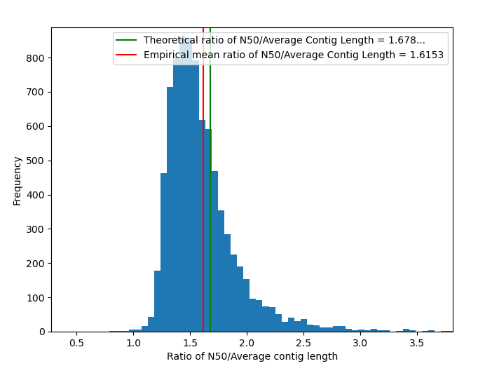
It turns out that the predicted N50/Average length ratio is about 3.4 percent off from the empirical value. Considering how often and how badly theoretical models fail in bioinformatics, I’ll consider this a win :).