In our (me and Yun William Yu’s) new paper “Seed-chain-extend alignment is accurate and runs in close to O(m log n) time for similar sequences: a rigorous average-case analysis”, we give rigorous bounds on seed-chain-extend alignment using average-case analysis on random, mutating strings. This blog post is meant to be:

1. A high-level exposition of the main ideas of the paper for people somewhat familiar with k-mers, alignment, and chaining.
2. An intuitive proof sketch of the runtime being close to \(O(m \log n).\)

Main motivation

Optimal alignment in the theoretical worse case is difficult; it takes \(O(mn)\) time for sequences of length \(n\) and \(m\) where \(m < n\) using e.g. Needleman-Wunsch or Smith-Waterman. Real aligners don’t just align reads or two genomes together using an \(O(mn)\) algorithm but use heuristics instead.

A popular heuristic used for alignment by aligners like minimap2 is k-mer seed-chain-extend, which uses k-mer seeds to approximately find an alignment. I’ll assume familiarity with what a chain of k-mer anchors is from now on. If you’re not familiar, I highly recommend the recent review article “A survey of mapping algorithms in the long-reads era”.

However, seed-chain-extend is still \(O(mn)\) in the worst-case: consider two strings \(S = AAAAA...\) and \(S' = AAAAA....\) of length \(n\) and \(m\); there will be \(O(mn)\) k-mer matches in this case, so finding all anchors already takes \(O(mn)\) time. Furthermore, there is no guarantee that the resulting alignment is optimal (although the chain may be optimal). In practice, however, the runtime is much better than \(O(mn)\) and the alignment usually works out okay.

Therefore, in order to break through the \(O(mn)\) runtime barrier, we use average-case analysis instead. This means we take the expected runtime over all possible inputs under some probabilistic model on our inputs. The idea is that as long as the inputs are not of the form \(AAAAA...\) too often under our random model, we can still do better than \(O(mn)\) on average.

Random input model

To do average-case analysis, we need a random model on our inputs to take an expectation over. When we align sequences, we generally believe there is some similarity between them, so aligning two random strings isn’t the correct model. We instead use an independent substitution model. We let \(S\) be a random string, and \(S'\) be a mutated substring of \(S\) where we take a substring of \(S\) and then mutate each character to a different letter with probability \(\theta\). The length of \(S\) is \(\sim n\) and \(S'\) is \(\sim m\) where \(\sim\) hides factors of \(k\) lurking around; see Section 2 for clarification.

We don’t model indels, but such independent substitution models have been used before to model k-mer statistics relatively well (e.g. mash). In my opinion, the much bigger issue is that repeats aren’t correctly modeled; if someone wants to take a stab at modeling random mutating string models with repeats, let me know!

What did we prove?

There are three main things we prove in the paper. Remember, \(m < n\) and \(\theta\) is the mutation rate of our string.

1. Expected runtime of extension is \(O(m n^{f(\theta)} \log n)\) for some \(f(\theta)\). It turns out \(f(\theta) < 0.08\) when \(\theta = 0.05\); see Supplementary Figure 7 for explicit \(f(\theta)\). This dominates the overall runtime.
2. Expected runtime of chaining is \(O(m \log m)\) (actually slightly better; see Theorem 1 in our paper).
3. Expected accuracy of resulting alignment: we can recover more than \(1 - O(1/\sqrt m)\) fraction of the “homologous” bases that are related.

In summary, we prove that the expected runtime is much better than \(O(mn)\) and actually give a result on alignment accuracy, which I don’t think has been done before. We also prove some things about sketched versions with k-mer subsampling, but I won’t discuss that here.

The chaining result (2) involves messing around with statistics of k-mers and that there are not too many k-mer hits. It’s an argument on mutating substring matching with a few technical lemmas. The accuracy result (3) is more messy to define and prove, and a lot of effort was dedicated to this. Both involve a mix of probabilistic and combinatorial tools. I won’t touch on what it means to be able to recover homologous bases here; see Section 4 if you’re interested.

I think the extension result (1) is the most interesting, and the main idea behind the proof is relatively simple. I’ll spend the rest of the blog talking about this result.

Core assumptions on seed-chain-extend

I will spend the rest of this blog explaining the main idea behind result (1) above.

In Section 2 of our paper, we go through our exact model seed-chain-extend. I’ll list the most important points below.

1. We let \(k = C \log n\) for some constant \(2 < C < 3\) which depends on only \(\theta\), and \(n\) is the size of the reference. So \(k\), the k-mer length, is increasing as the genome size increases. \(C\) is defined in Theorem 1 in our paper.
2. We use fixed length k-mer seeds. Anchors are exact matches of k-mers. Assume no sketching in this blog post.
3. We use a linear gap cost and solve it in \(O(N \log N)\) time where \(N\) is the number of anchors. See for example minigraph for the definition of linear gap cost and the \(O(N \log N)\) range-min/max-query solution. This isn’t important for the rest of my post, but the linear gap cost is used in the paper to prove some of the assumptions I list below. In principle, any gap cost that penalizes large gaps should work, but you can’t ignore gaps (i.e. don’t just take the chain with most anchors).
4. k-mer anchors are allowed to overlap. If you’re experienced with chaining, you know that allowing overlaps without explicitly accounting for overlaps in the cost may not model the chain properly. For us, however, it is mathematically convenient to allow overlaps.
5. We perform quadratic time extension between gaps in the resulting chain. We don’t actually care about the cost (e.g. edit, affine, dual-affine, …) for this.

How do we prove extension is fast?

Intuitively, we just want to show that the gaps between anchors in the resulting chain are small and not plentiful. Remember that the resulting chain is now random since our inputs are random. The optimal chain can be kind of weird, so we look at the longest homologous chain, which I define below.

In the following image, vertical bases are derived from the same ancestral sequence, and grey bases are mutated. The blue k-mer anchors come from positions that are hence homologous, whereas the red anchors are spurious anchors resulting from randomness. The alignment matrix in the bottom panel shows how k-mer matches look when considering a dynamic programming matrix.

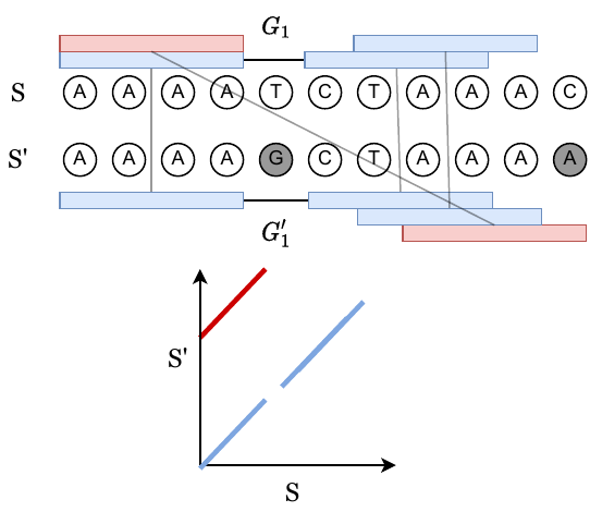
We can always obtain a chain by just taking all blue, homologous anchors. Let’s call this the homologous chain.

Claim: The homologous chain may not be optimal, but in our paper, we prove that the runtime through the possibly non-optimal homologous chain is the dominant big O term.

The above claim takes quite a bit of work, but I think it’s relatively believable. Intuitively, we pick \(k = C \log n\) big enough such that spurious anchors don’t happen too often. The homologous chain is much, much easier to work with than an arbitrary optimal chain, so our problem becomes much easier now.

Modeling gaps between homologous k-mers

The following sections are a high-level version of Appendix D.5 in our paper.

In the above figure, we have a gap labeled \(G_1\). These are also called “islands”, and the number of islands that appear in a random mutating sequence is studied in “The Statistics of k-mers from a Sequence Undergoing a Simple Mutation Process Without Spurious Matches. Our problem is slightly different since we want the length of the islands, and not just the number of islands.

Assuming we have gaps \(G_1, G_2, ...\), the runtime of extension is \(O(G_1^2) + O(G_2^2) + ...\) because it takes quadratic time to extend through gaps. Alternatively, the dynamic programming matrix induced by the gap of size \(G_1\) is of size \(G_1^2\). However, the \(G_i\)s are random variables, so we want \(O(\mathbb{E} [G_1^2]) + O(\mathbb{E}[G_2^2]) + ...\) The number of \(G_i\)s is also random variable, so calculating this sum directly is challenging.

Definition: To model gaps properly, let us instead define a random variable \(Y_i\) where \(Y_i = \ell > 0\) if

1. the k-mer starting at position \(i\) is unmutated (none of its bases are mutated)
2. and the k-mer starting at position \(i + \ell + k\) is unmutated
3. and no k-mers between these two flanking k-mers are unmutated (i.e. they’re all mutated).

If any of these conditions fail, \(Y_i = 0\).

It’s not too hard to see that \(Y_i\) represents the size of a gap starting at position \(i+k\) if and only if a gap of size \(>0\) exists, and is \(0\) otherwise. In particular, the \(G_i\)s are in 1-to-1 correspondence with non-zero \(Y_i\)s, so

We sum up to \(m\) because there are \(m\) homologous k-mers since \(m < n\). But now, the number of \(Y_i\)s is no longer a random variable! So we can just take expectations and use linearity of expectation to get a result.

Making k-mers independent as an upper bound.

We’re almost there, but not quite yet. We do a trick to upper bound \(Y_1^2 + ... + Y_m^2\). The problem is that in conditions (1), (2), and (3) above, the k-mers are not independent. Precisely, the “k-mers between these two flanking k-mers” in (3) share bases with the flanking k-mers, so they’re dependent under our mutation model.

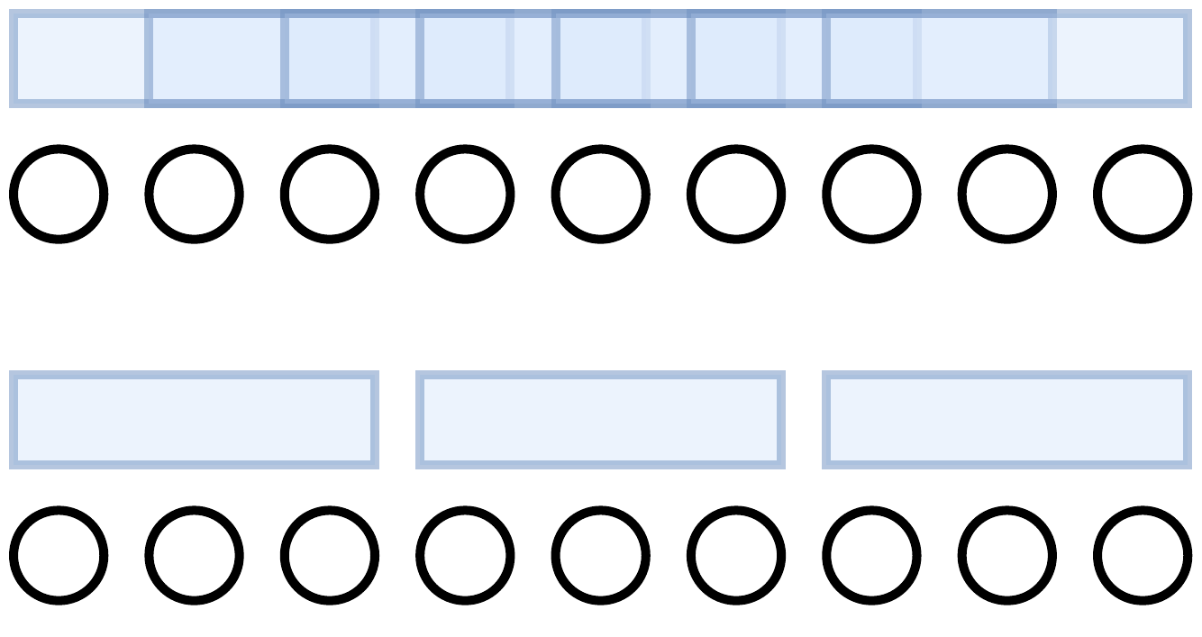
To remove this dependence, we instead only consider k-mers that are spaced exactly k bases apart. That is, let \(K\) be a maximal set of k-mers spaced exactly \(k\) bases apart from each other. k-mers in \(K\) do not overlap at all. The bottom set of k-mers in the below picture is \(K\).

Definition: Now let \(Y_i^K\) be the random variable such that \(Y_i^K = x\) if

1. the k-mer starting at position \(i\) is unmutated (none of its bases are mutated) and this k-mer is in \(K\)
2. and the k-mer starting at position \(i + x + k\) is unmutated and this k-mer is in \(K\)
3. and no k-mers in \(K\) between these two flanking k-mers are unmutated (i.e. they’re all mutated).

And we let \(Y_i^K = 0\) if any of these conditions are violated. \(Y_i^K\)s represent the gaps when only considering k-mers in \(K\).

Claim: It should be intuitively obvious that the gaps are larger when only considering k-mers in \(K\) instead of all k-mers, thus we get an upper bound by considering \(Y_i^K\)s; we prove this more rigorously in Appendix D.5.

Thus we are left with bounding

Recall that \(m\) is the size of \(S'\) (modulo factors of \(k\), which are small), the smaller string. Now we can see that all except for about \(m/k\) of the \(Y_i^K\) are always \(0\) since there are only \(m/k\) k-mers in \(K\), so only \(m/k\) of the random variables satisfy condition (1) above.

Calculating expectation of \((Y_i^K)^2\).

Let’s compute \(\Pr(Y_i^K = x)\). I claim that assuming the k-mer at \(i\) is in \(K\),

Firstly, \(Y_i^K\) can not equal non-multiples of \(k\) by our construction. The first \((1-\theta)^k\) comes from condition (1) above, and the second follows from condition (2). The probability a k-mer is unmutated is \((1-\theta)^k\) because all mutations are independent. The last term comes from the fact that if there are \(\ell \cdot k\) bases between the first and last k-mer, there are exactly \(\ell\) k-mers in between them (in \(K\)). These k-mers are independent, so the probability that all of them are mutated is \((1 - (1-\theta)^k)^\ell\). The \(\leq\) follows because the gap size can not be greater than \(m\), so the actual value would be 0 in that case.

Now we can finally calculate what we wanted, which is \(\mathbb{E}[(Y_i^K)^2]\). This is

We only sum over \(\ell\), so this is

Geometric series calculus (or Mathematica) tells us that \(\sum_{i=1}^\infty i^2 x^i = \frac{x (x+1)}{(1-x)^3}\) (there’s a typo in version 1 of our paper on pg. 28; this is the correct formula). Thus plugging this in, we get

after remembering that \((1-\theta)^k = o(1)\) because we assumed that \(k = C \log n\) way back for some constant \(C\). Now recall there are \(m/k\) non-zero \(Y_i^K\) random variables, so our final number of gaps squared is

After a final substitution of \(k = C \log n\), we get that

where \(-C \log (1 - \theta) = f (\theta)\), and we’re done. In the paper, we take \(C \sim \frac{2}{1 + 2 \log(1-\theta)}\) for reasons relating to the accuracy result, so \(C\) actually depends on \(\theta\) as well.

Conclusion

We showed that the runtime of extending through the gaps in the homologous chain of k-mers is \(O(m n^{f(\theta)} \log n )\), which is almost \(O(m \log n)\) when \(\theta\) is small. For example, we can explicit calculate \(f(0.05) < 0.08\) when \(\theta\) is \(0.05\), so the runtime in this case this is \(O(m n^{0.08} \log n)\). \(n^{0.08}\) is actually smaller than \(\log n\) when \(n < 10^{21}\), so it’s really, really small for realistic \(n\).

Remember, I did not claim that we’re actually aligning through the homologous chain; we’re aligning through the optimal chain given by linear gap cost chaining. However, in the paper, we show that the actual runtime is dominated by this homologous chain extension runtime. This shouldn’t be too head-scratching; most of the time (especially without repeats), we expect the correct chain to be the obvious, homologous one. It’s surprisingly challenging to prove, though, and comes down to bounding breaks, which I won’t go into here.

Last thought I’d like to mention: one of the punchlines of our paper involves sketching. We show that this same bound holds even when we subsample the k-mers. The proof for that result follows the same intuition as this proof, but it actually uses a non-independent Chernoff bound to bound the \(Y_i\)s instead, leading to some slightly different techniques.